0. before you start
1. getting started
2. the @cortex class
3. creating a @cortex object
4. things you do with a @cortex object
5. the @key class
6. creating a @key object
7. the key file
8. working with @key objects
9. using @cortex and @key objects
10. spike data analysis
11. the @spix class

10. Spike data analysis

Spikes occurring within the epochs specified in the @key can be counted and averaged using a small set of @cortex methods. The mother (or father?) of all such methods is:

spikematrix

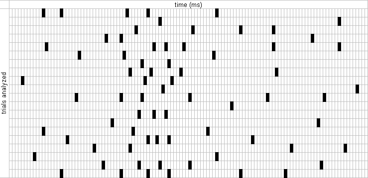
This function returns an m-by-n matrix, where each m corresponds to a single time window selected for analysis, and each n represents 1 ms. Elements in the matrix can only be zeros and ones. A value of 1 indicates the occurrence of a spike. The figure below helps visualize a spikematrix. This is how to call spikematrix:

>> [spmat, trials] = spikematrix(c, s, k);

where c is the @cortex object, s is the spike to analyze, and k is a single key (either simple or complex) from a @key object. The return argument trials is a m-by-1 array with the trial number corresponding to each spmat row.

trialfiringrate and meanfiringrate

A very common task is to compute firing rates (in spikes per second), for subsets of experimental trials, over meaningful time windows. The function trialfiringrate returns spike-per-second rates for the trials selected and over the epoch specified by a key. Do:

>> help cortex/trialfiringrate for more details.

To average firing rates across trials that "belong together" use the function meanfiringrate. Do:

>> help cortex/meanfiringrate for more details.

Note that both trialfiringrate and meanfiringrate internally call spikematrix.

plotting neuronal activity

Spike density plots are a common way to visualize a neuron's firing activity over time. The function density computes "smoothed" firing rates, and its output can be directly plotted on a chart.

>> c = cortex ('040502.0', 1:2);
>> k = key ('keys.key');
>> spike = c.bank(1);
>> kwidth = 10; % convolution kernel width in ms
>> d = density (c, spike, kwidth, 'gauss', k(1));
>> plot (d)

Previous <-> Next